
Final Up to date on September 25, 2019
The chance for a steady random variable could be summarized with a steady chance distribution.
Steady chance distributions are encountered in machine studying, most notably within the distribution of numerical enter and output variables for fashions and within the distribution of errors made by fashions. Information of the conventional steady chance distribution can also be required extra usually within the density and parameter estimation carried out by many machine studying fashions.
As such, steady chance distributions play an vital function in utilized machine studying and there are just a few distributions {that a} practitioner should find out about.
On this tutorial, you’ll uncover steady chance distributions utilized in machine studying.
After finishing this tutorial, you’ll know:
- The chance of outcomes for steady random variables could be summarized utilizing steady chance distributions.
- Tips on how to parametrize, outline, and randomly pattern from widespread steady chance distributions.
- Tips on how to create chance density and cumulative density plots for widespread steady chance distributions.
Kick-start your venture with my new e-book Chance for Machine Studying, together with step-by-step tutorials and the Python supply code recordsdata for all examples.
Let’s get began.

Steady Chance Distributions for Machine Studying
Picture by Bureau of Land Administration, some rights reserved.
Tutorial Overview
This tutorial is split into 4 elements; they’re:
- Steady Chance Distributions
- Regular Distribution
- Exponential Distribution
- Pareto Distribution
Steady Chance Distributions
A random variable is a amount produced by a random course of.
A steady random variable is a random variable that has an actual numerical worth.
Every numerical consequence of a steady random variable could be assigned a chance.
The connection between the occasions for a steady random variable and their possibilities is known as the continual chance distribution and is summarized by a chance density operate, or PDF for brief.
In contrast to a discrete random variable, the chance for a given steady random variable can’t be specified instantly; as an alternative, it’s calculated as an integral (space beneath the curve) for a tiny interval across the particular consequence.
The chance of an occasion equal to or lower than a given worth is outlined by the cumulative distribution operate, or CDF for brief. The inverse of the CDF is known as the percentage-point operate and can give the discrete consequence that’s lower than or equal to a chance.
- PDF: Chance Density Operate, returns the chance of a given steady consequence.
- CDF: Cumulative Distribution Operate, returns the chance of a worth lower than or equal to a given consequence.
- PPF: %-Level Operate, returns a discrete worth that’s lower than or equal to the given chance.
There are lots of widespread steady chance distributions. The commonest is the conventional chance distribution. Virtually all steady chance distributions of curiosity belong to the so-called exponential household of distributions, that are only a assortment of parameterized chance distributions (e.g. distributions that change primarily based on the values of parameters).
Steady chance distributions play an vital function in machine studying from the distribution of enter variables to the fashions, the distribution of errors made by fashions, and within the fashions themselves when estimating the mapping between inputs and outputs.
Within the following sections, will take a more in-depth take a look at among the extra widespread steady chance distributions.
Need to Be taught Chance for Machine Studying
Take my free 7-day e mail crash course now (with pattern code).
Click on to sign-up and likewise get a free PDF E book model of the course.
Regular Distribution
The regular distribution can also be known as the Gaussian distribution (named for Carl Friedrich Gauss) or the bell curve distribution.
The distribution covers the chance of real-valued occasions from many various drawback domains, making it a standard and well-known distribution, therefore the title “regular.” A steady random variable that has a standard distribution is claimed to be “regular” or “usually distributed.”
Some examples of domains which have usually distributed occasions embrace:
- The heights of individuals.
- The weights of infants.
- The scores on a take a look at.
The distribution could be outlined utilizing two parameters:
- Imply (mu): The anticipated worth.
- Variance (sigma^2): The unfold from the imply.
Typically, the usual deviation is used as an alternative of the variance, which is calculated because the sq. root of the variance, e.g. normalized.
- Customary Deviation (sigma): The typical unfold from the imply.
A distribution with a imply of zero and a typical deviation of 1 is known as a typical regular distribution, and sometimes information is decreased or “standardized” to this for evaluation for ease of interpretation and comparability.
We are able to outline a distribution with a imply of fifty and a typical deviation of 5 and pattern random numbers from this distribution. We are able to obtain this utilizing the regular() NumPy operate.
The instance under samples and prints 10 numbers from this distribution.
|
# pattern a standard distribution from numpy.random import regular # outline the distribution mu = 50 sigma = 5 n = 10 # generate the pattern pattern = regular(mu, sigma, n) print(pattern) |
Working the instance prints 10 numbers randomly sampled from the outlined regular distribution.
|
[48.71009029 49.36970461 45.58247748 51.96846616 46.05793544 40.3903483 48.39189421 50.08693721 46.85896352 44.83757824] |
A pattern of knowledge could be checked to see whether it is random by plotting it and checking for the acquainted regular form, or through the use of statistical assessments. If the samples of observations of a random variable are usually distributed, then they are often summarized by simply the imply and variance, calculated instantly on the samples.
We are able to calculate the chance of every commentary utilizing the chance density operate. A plot of those values would give us the tell-tale bell form.
We are able to outline a standard distribution utilizing the norm() SciPy operate after which calculate properties such because the moments, PDF, CDF, and extra.
The instance under calculates the chance for integer values between 30 and 70 in our distribution and plots the outcome, then does the identical for the cumulative chance.
|
1 2 3 4 5 6 7 8 9 10 11 12 13 14 15 16 17 |
# pdf and cdf for a standard distribution from scipy.stats import norm from matplotlib import pyplot # outline distribution parameters mu = 50 sigma = 5 # create distribution dist = norm(mu, sigma) # plot pdf values = [value for value in range(30, 70)] possibilities = [dist.pdf(value) for value in values] pyplot.plot(values, possibilities) pyplot.present() # plot cdf cprobs = [dist.cdf(value) for value in values] pyplot.plot(values, cprobs) pyplot.present() |
Working the instance first calculates the chance for integers within the vary [30, 70] and creates a line plot of values and possibilities.
The plot exhibits the Gaussian or bell-shape with the height of highest chance across the anticipated worth or imply of fifty with a chance of about 8%.
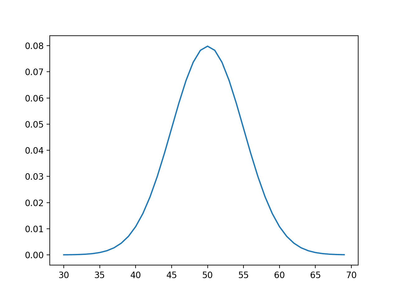
Line Plot of Occasions vs Chance or the Chance Density Operate for the Regular Distribution
The cumulative possibilities are then calculated for observations over the identical vary, displaying that on the imply, we have now lined about 50% of the anticipated values and really near 100% after the worth of about 65 or 3 normal deviations from the imply (50 + (3 * 5)).
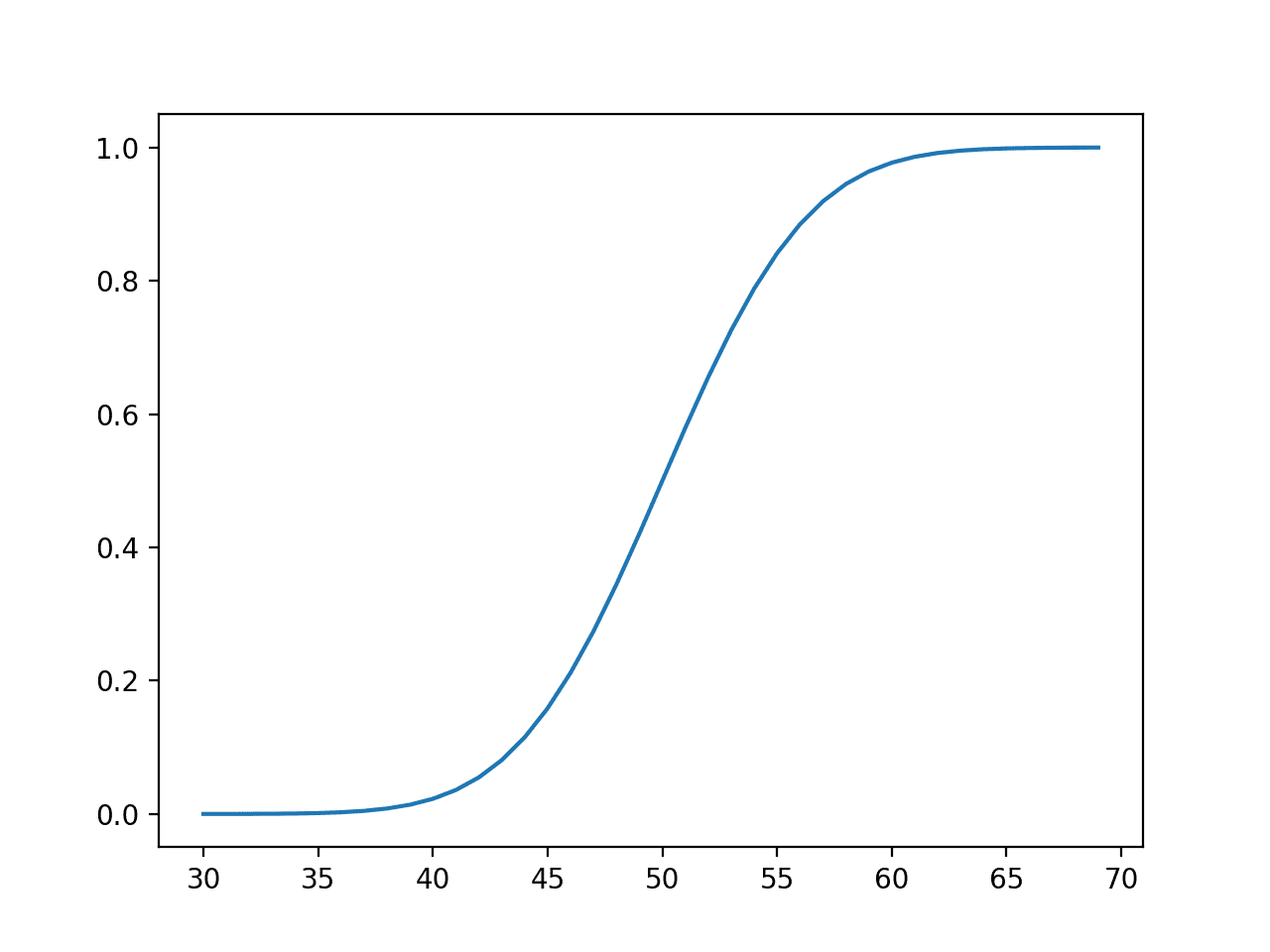
Line Plot of Occasions vs. Cumulative Chance or the Cumulative Density Operate for the Regular Distribution
In truth, the conventional distribution has a heuristic or rule of thumb that defines the share of knowledge lined by a given vary by the variety of normal deviations from the imply. It’s known as the 68-95-99.7 rule, which is the approximate proportion of the information lined by ranges outlined by 1, 2, and three normal deviations from the imply.
For instance, in our distribution with a imply of fifty and a typical deviation of 5, we’d count on 95% of the information to be lined by values which are 2 normal deviations from the imply, or 50 – (2 * 5) and 50 + (2 * 5) or between 40 and 60.
We are able to verify this by calculating the precise values utilizing the percentage-point operate.
The center 95% can be outlined by the share level operate worth for two.5% on the low finish and 97.5% on the excessive finish, the place 97.5 – 2.5 provides the center 95%.
The whole instance is listed under.
|
# calculate the values that outline the center 95% from scipy.stats import norm # outline distribution parameters mu = 50 sigma = 5 # create distribution dist = norm(mu, sigma) low_end = dist.ppf(0.025) high_end = dist.ppf(0.975) print(‘Center 95%% between %.1f and %.1f’ % (low_end, high_end)) |
Working the instance provides the precise outcomes that outline the center 95% of anticipated outcomes which are very near our standard-deviation-based heuristics of 40 and 60.
|
Center 95% between 40.2 and 59.8 |
An vital associated distribution is the Log-Regular chance distribution.
Exponential Distribution
The exponential distribution is a steady chance distribution the place just a few outcomes are the almost certainly with a fast lower in chance to all different outcomes.
It’s the steady random variable equal to the geometric chance distribution for discrete random variables.
Some examples of domains which have exponential distribution occasions embrace:
- The time between clicks on a Geiger counter.
- The time till the failure of a component.
- The time till the default of a mortgage.
The distribution could be outlined utilizing one parameter:
- Scale (Beta): The imply and normal deviation of the distribution.
Typically the distribution is outlined extra formally with a parameter lambda or charge. The beta parameter is outlined because the reciprocal of the lambda parameter (beta = 1/lambda)
- Fee (lambda) = Fee of change within the distribution.
We are able to outline a distribution with a imply of fifty and pattern random numbers from this distribution. We are able to obtain this utilizing the exponential() NumPy operate.
The instance under samples and prints 10 numbers from this distribution.
|
# pattern an exponential distribution from numpy.random import exponential # outline the distribution beta = 50 n = 10 # generate the pattern pattern = exponential(beta, n) print(pattern) |
Working the instance prints 10 numbers randomly sampled from the outlined distribution.
|
[ 3.32742946 39.10165624 41.86856606 85.0030387 28.18425491 68.20434637 106.34826579 19.63637359 17.13805423 15.91135881] |
We are able to outline an exponential distribution utilizing the expon() SciPy operate after which calculate properties such because the moments, PDF, CDF, and extra.
The instance under defines a spread of observations between 50 and 70 and calculates the chance and cumulative chance for every and plots the outcome.
|
# pdf and cdf for an exponential distribution from scipy.stats import expon from matplotlib import pyplot # outline distribution parameter beta = 50 # create distribution dist = expon(beta) # plot pdf values = [value for value in range(50, 70)] possibilities = [dist.pdf(value) for value in values] pyplot.plot(values, possibilities) pyplot.present() # plot cdf cprobs = [dist.cdf(value) for value in values] pyplot.plot(values, cprobs) pyplot.present() |
Working the instance first creates a line plot of outcomes versus possibilities, displaying a well-known exponential chance distribution form.
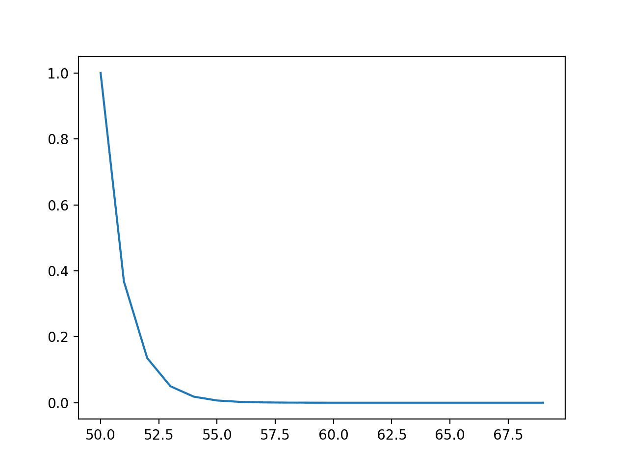
Line Plot of Occasions vs. Chance or the Chance Density Operate for the Exponential Distribution
Subsequent, the cumulative possibilities for every consequence are calculated and graphed as a line plot, displaying that after maybe a worth of 55 that nearly 100% of the anticipated values can be noticed.
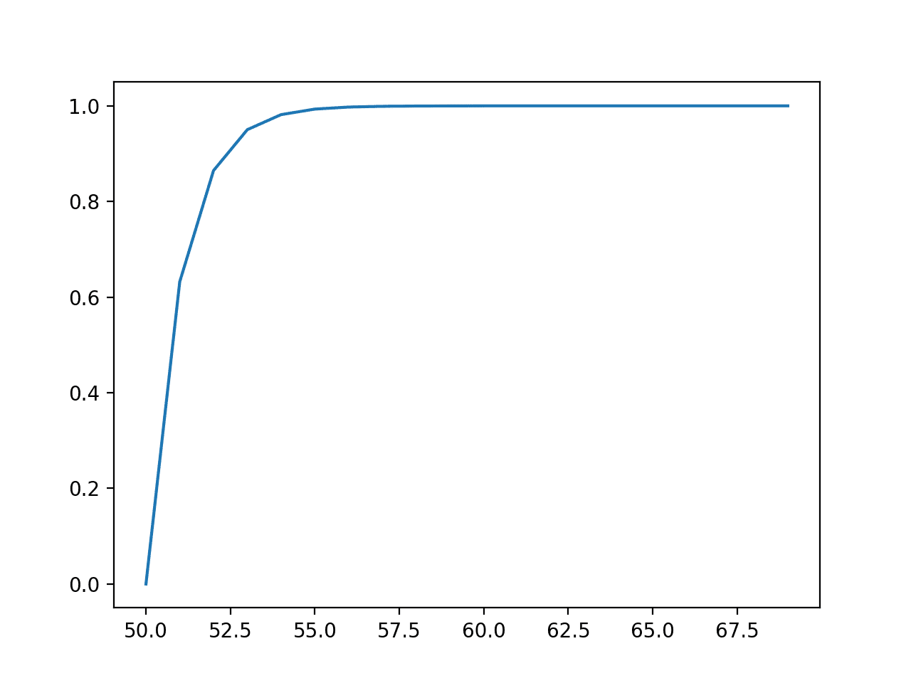
Line Plot of Occasions vs. Cumulative Chance or the Cumulative Density Operate for the Exponential Distribution
An vital associated distribution is the double exponential distribution, additionally known as the Laplace distribution.
Pareto Distribution
A Pareto distribution is known as after Vilfredo Pareto and is could also be known as a power-law distribution.
Additionally it is associated to the Pareto precept (or 80/20 rule) which is a heuristic for steady random variables that comply with a Pareto distribution, the place 80% of the occasions are lined by 20% of the vary of outcomes, e.g. most occasions are drawn from simply 20% of the vary of the continual variable.
The Pareto precept is only a heuristic for a particular Pareto distribution, particularly the Pareto Kind II distribution, that’s maybe most attention-grabbing and on which we’ll focus.
Some examples of domains which have Pareto distributed occasions embrace:
- The earnings of households in a rustic.
- The whole gross sales of books.
- The scores by gamers on a sports activities staff.
The distribution could be outlined utilizing one parameter:
- Form (alpha): The steepness of the decease in chance.
Values for the form parameter are sometimes small, reminiscent of between 1 and three, with the Pareto precept given when alpha is about to 1.161.
We are able to outline a distribution with a form of 1.1 and pattern random numbers from this distribution. We are able to obtain this utilizing the pareto() NumPy operate.
|
# pattern a pareto distribution from numpy.random import pareto # outline the distribution alpha = 1.1 n = 10 # generate the pattern pattern = pareto(alpha, n) print(pattern) |
Working the instance prints 10 numbers randomly sampled from the outlined distribution.
|
[0.5049704 0.0140647 2.13105224 3.10991217 2.87575892 1.06602639 0.22776379 0.37405415 0.96618778 3.94789299] |
We are able to outline a Pareto distribution utilizing the pareto() SciPy operate after which calculate properties, such because the moments, PDF, CDF, and extra.
The instance under defines a spread of observations between 1 and about 10 and calculates the chance and cumulative chance for every and plots the outcome.
|
# pdf and cdf for a pareto distribution from scipy.stats import pareto from matplotlib import pyplot # outline distribution parameter alpha = 1.5 # create distribution dist = pareto(alpha) # plot pdf values = [value/10.0 for value in range(10, 100)] possibilities = [dist.pdf(value) for value in values] pyplot.plot(values, possibilities) pyplot.present() # plot cdf cprobs = [dist.cdf(value) for value in values] pyplot.plot(values, cprobs) pyplot.present() |
Working the instance first creates a line plot of outcomes versus possibilities, displaying a well-known Pareto chance distribution form.
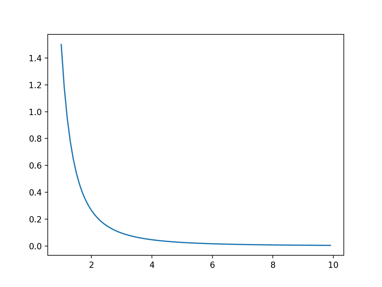
Line Plot of Occasions vs. Chance or the Chance Density Operate for the Pareto Distribution
Subsequent, the cumulative possibilities for every consequence are calculated and graphed as a line plot, displaying an increase that’s much less steep than the exponential distribution seen within the earlier part.
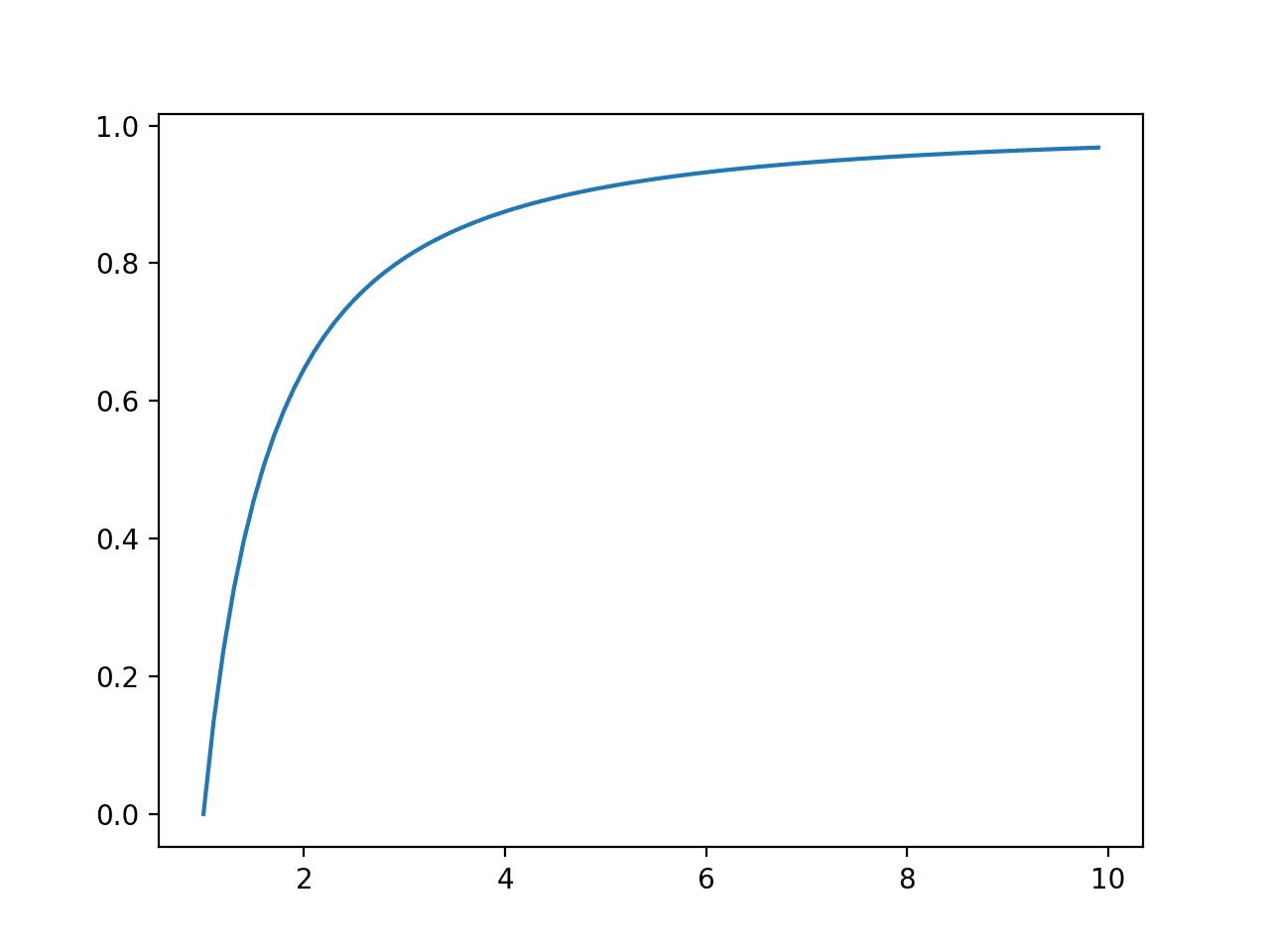
Line Plot of Occasions vs. Cumulative Chance or the Cumulative Density Operate for the Pareto Distribution
Additional Studying
This part supplies extra sources on the subject if you’re trying to go deeper.
Books
API
Articles
Abstract
On this tutorial, you found steady chance distributions utilized in machine studying.
Particularly, you discovered:
- The chance of outcomes for steady random variables could be summarized utilizing steady chance distributions.
- Tips on how to parametrize, outline, and randomly pattern from widespread steady chance distributions.
- Tips on how to create chance density and cumulative density plots for widespread steady chance distributions.
Do you’ve gotten any questions?
Ask your questions within the feedback under and I’ll do my greatest to reply.
Get a Deal with on Chance for Machine Studying!
Develop Your Understanding of Chance
…with only a few traces of python code
Uncover how in my new E book:
Chance for Machine Studying
It supplies self-study tutorials and end-to-end tasks on:
Bayes Theorem, Bayesian Optimization, Distributions, Most Chance, Cross-Entropy, Calibrating Fashions
and way more…
Lastly Harness Uncertainty in Your Tasks
Skip the Teachers. Simply Outcomes.