
Final Up to date on November 2, 2022
We now have put collectively the full Transformer mannequin, and now we’re prepared to coach it for neural machine translation. We will use a coaching dataset for this function, which comprises quick English and German sentence pairs. We can even revisit the position of masking in computing the accuracy and loss metrics in the course of the coaching course of.
On this tutorial, you’ll uncover methods to prepare the Transformer mannequin for neural machine translation.
After finishing this tutorial, you’ll know:
- How one can put together the coaching dataset
- How one can apply a padding masks to the loss and accuracy computations
- How one can prepare the Transformer mannequin
Let’s get began.

Coaching the transformer mannequin
Picture by v2osk, some rights reserved.
Tutorial Overview
This tutorial is split into 4 components; they’re:
- Recap of the Transformer Structure
- Making ready the Coaching Dataset
- Making use of a Padding Masks to the Loss and Accuracy Computations
- Coaching the Transformer Mannequin
Conditions
For this tutorial, we assume that you’re already accustomed to:
Recap of the Transformer Structure
Recall having seen that the Transformer structure follows an encoder-decoder construction. The encoder, on the left-hand facet, is tasked with mapping an enter sequence to a sequence of steady representations; the decoder, on the right-hand facet, receives the output of the encoder along with the decoder output on the earlier time step to generate an output sequence.
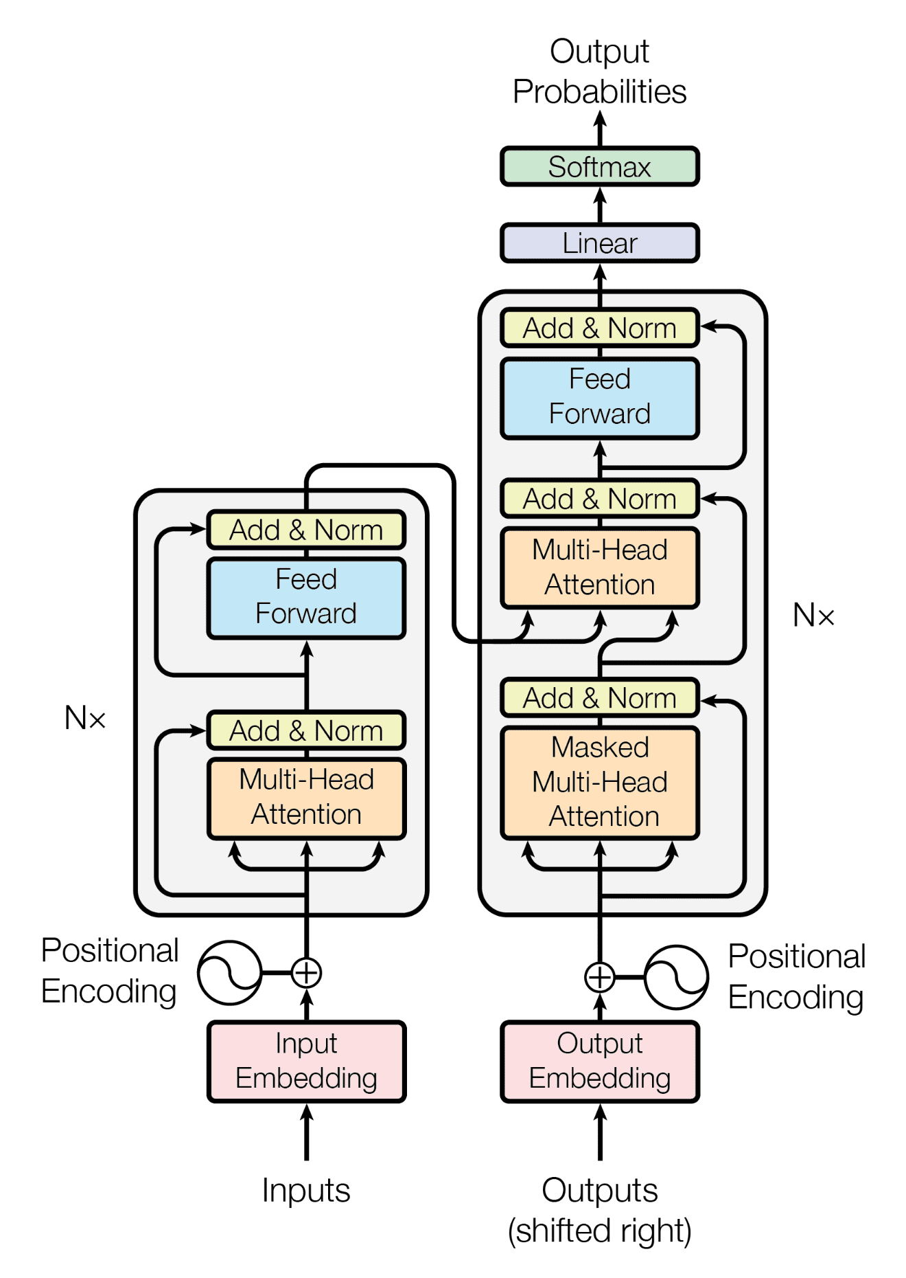
The encoder-decoder construction of the Transformer structure
Taken from “Consideration Is All You Want“
In producing an output sequence, the Transformer doesn’t depend on recurrence and convolutions.
You have got seen methods to implement the entire Transformer mannequin, so now you can proceed to coach it for neural machine translation.
Let’s begin first by getting ready the dataset for coaching.
Kick-start your mission with my guide Constructing Transformer Fashions with Consideration. It gives self-study tutorials with working code to information you into constructing a fully-working transformer fashions that may
translate sentences from one language to a different…
Making ready the Coaching Dataset
For this function, you’ll be able to confer with a earlier tutorial that covers materials about getting ready the textual content information for coaching.
Additionally, you will use a dataset that comprises quick English and German sentence pairs, which you will obtain right here. This specific dataset has already been cleaned by eradicating non-printable and non-alphabetic characters and punctuation characters, additional normalizing all Unicode characters to ASCII, and altering all uppercase letters to lowercase ones. Therefore, you’ll be able to skip the cleansing step, which is usually a part of the information preparation course of. Nonetheless, should you use a dataset that doesn’t come readily cleaned, you’ll be able to confer with this this earlier tutorial to find out how to take action.
Let’s proceed by creating the PrepareDataset class that implements the next steps:
- Hundreds the dataset from a specified filename.
|
clean_dataset = load(open(filename, ‘rb’)) |
- Selects the variety of sentences to make use of from the dataset. Because the dataset is giant, you’ll cut back its dimension to restrict the coaching time. Nonetheless, you might discover utilizing the total dataset as an extension to this tutorial.
|
dataset = clean_dataset[:self.n_sentences, :] |
- Appends begin (<START>) and end-of-string (<EOS>) tokens to every sentence. For instance, the English sentence,
i prefer to run, now turns into,<START> i prefer to run <EOS>. This additionally applies to its corresponding translation in German,ich gehe gerne joggen, which now turns into,<START> ich gehe gerne joggen <EOS>.
|
for i in vary(dataset[:, 0].dimension): dataset[i, 0] = “<START> “ + dataset[i, 0] + ” <EOS>” dataset[i, 1] = “<START> “ + dataset[i, 1] + ” <EOS>” |
- Shuffles the dataset randomly.
- Splits the shuffled dataset based mostly on a pre-defined ratio.
|
prepare = dataset[:int(self.n_sentences * self.train_split)] |
- Creates and trains a tokenizer on the textual content sequences that will likely be fed into the encoder and finds the size of the longest sequence in addition to the vocabulary dimension.
|
enc_tokenizer = self.create_tokenizer(prepare[:, 0]) enc_seq_length = self.find_seq_length(prepare[:, 0]) enc_vocab_size = self.find_vocab_size(enc_tokenizer, prepare[:, 0]) |
- Tokenizes the sequences of textual content that will likely be fed into the encoder by making a vocabulary of phrases and changing every phrase with its corresponding vocabulary index. The <START> and <EOS> tokens can even type a part of this vocabulary. Every sequence can also be padded to the utmost phrase size.
|
trainX = enc_tokenizer.texts_to_sequences(prepare[:, 0]) trainX = pad_sequences(trainX, maxlen=enc_seq_length, padding=‘publish’) trainX = convert_to_tensor(trainX, dtype=int64) |
- Creates and trains a tokenizer on the textual content sequences that will likely be fed into the decoder, and finds the size of the longest sequence in addition to the vocabulary dimension.
|
dec_tokenizer = self.create_tokenizer(prepare[:, 1]) dec_seq_length = self.find_seq_length(prepare[:, 1]) dec_vocab_size = self.find_vocab_size(dec_tokenizer, prepare[:, 1]) |
- Repeats an analogous tokenization and padding process for the sequences of textual content that will likely be fed into the decoder.
|
trainY = dec_tokenizer.texts_to_sequences(prepare[:, 1]) trainY = pad_sequences(trainY, maxlen=dec_seq_length, padding=‘publish’) trainY = convert_to_tensor(trainY, dtype=int64) |
The entire code itemizing is as follows (confer with this earlier tutorial for additional particulars):
|
1 2 3 4 5 6 7 8 9 10 11 12 13 14 15 16 17 18 19 20 21 22 23 24 25 26 27 28 29 30 31 32 33 34 35 36 37 38 39 40 41 42 43 44 45 46 47 48 49 50 51 52 53 54 55 56 57 58 59 60 61 62 63 64 65 66 67 |
from pickle import load from numpy.random import shuffle from keras.preprocessing.textual content import Tokenizer from keras.preprocessing.sequence import pad_sequences from tensorflow import convert_to_tensor, int64
class PrepareDataset: def __init__(self, **kwargs): tremendous(PrepareDataset, self).__init__(**kwargs) self.n_sentences = 10000 # Variety of sentences to incorporate within the dataset self.train_split = 0.9 # Ratio of the coaching information break up
# Match a tokenizer def create_tokenizer(self, dataset): tokenizer = Tokenizer() tokenizer.fit_on_texts(dataset)
return tokenizer
def find_seq_length(self, dataset): return max(len(seq.break up()) for seq in dataset)
def find_vocab_size(self, tokenizer, dataset): tokenizer.fit_on_texts(dataset)
return len(tokenizer.word_index) + 1
def __call__(self, filename, **kwargs): # Load a clear dataset clean_dataset = load(open(filename, ‘rb’))
# Scale back dataset dimension dataset = clean_dataset[:self.n_sentences, :]
# Embody begin and finish of string tokens for i in vary(dataset[:, 0].dimension): dataset[i, 0] = “<START> “ + dataset[i, 0] + ” <EOS>” dataset[i, 1] = “<START> “ + dataset[i, 1] + ” <EOS>”
# Random shuffle the dataset shuffle(dataset)
# Break up the dataset prepare = dataset[:int(self.n_sentences * self.train_split)]
# Put together tokenizer for the encoder enter enc_tokenizer = self.create_tokenizer(prepare[:, 0]) enc_seq_length = self.find_seq_length(prepare[:, 0]) enc_vocab_size = self.find_vocab_size(enc_tokenizer, prepare[:, 0])
# Encode and pad the enter sequences trainX = enc_tokenizer.texts_to_sequences(prepare[:, 0]) trainX = pad_sequences(trainX, maxlen=enc_seq_length, padding=‘publish’) trainX = convert_to_tensor(trainX, dtype=int64)
# Put together tokenizer for the decoder enter dec_tokenizer = self.create_tokenizer(prepare[:, 1]) dec_seq_length = self.find_seq_length(prepare[:, 1]) dec_vocab_size = self.find_vocab_size(dec_tokenizer, prepare[:, 1])
# Encode and pad the enter sequences trainY = dec_tokenizer.texts_to_sequences(prepare[:, 1]) trainY = pad_sequences(trainY, maxlen=dec_seq_length, padding=‘publish’) trainY = convert_to_tensor(trainY, dtype=int64)
return trainX, trainY, prepare, enc_seq_length, dec_seq_length, enc_vocab_size, dec_vocab_size |
Earlier than shifting on to coach the Transformer mannequin, let’s first take a look on the output of the PrepareDataset class similar to the primary sentence within the coaching dataset:
|
# Put together the coaching information dataset = PrepareDataset() trainX, trainY, train_orig, enc_seq_length, dec_seq_length, enc_vocab_size, dec_vocab_size = dataset(‘english-german-both.pkl’)
print(train_orig[0, 0], ‘n’, trainX[0, :]) |
|
<START> did tom let you know <EOS> tf.Tensor([ 1 25 4 97 5 2 0], form=(7,), dtype=int64) |
(Be aware: Because the dataset has been randomly shuffled, you’ll possible see a special output.)
You possibly can see that, initially, you had a three-word sentence (did tom let you know) to which you appended the beginning and end-of-string tokens. Then you definitely proceeded to vectorize (you might discover that the <START> and <EOS> tokens are assigned the vocabulary indices 1 and a couple of, respectively). The vectorized textual content was additionally padded with zeros, such that the size of the top consequence matches the utmost sequence size of the encoder:
|
print(‘Encoder sequence size:’, enc_seq_length) |
|
Encoder sequence size: 7 |
You possibly can equally try the corresponding goal information that’s fed into the decoder:
|
print(train_orig[0, 1], ‘n’, trainY[0, :]) |
|
<START> hat tom es dir gesagt <EOS> tf.Tensor([ 1 14 5 7 42 162 2 0 0 0 0 0], form=(12,), dtype=int64) |
Right here, the size of the top consequence matches the utmost sequence size of the decoder:
|
print(‘Decoder sequence size:’, dec_seq_length) |
|
Decoder sequence size: 12 |
Making use of a Padding Masks to the Loss and Accuracy Computations
Recall seeing that the significance of getting a padding masks on the encoder and decoder is to ensure that the zero values that we now have simply appended to the vectorized inputs aren’t processed together with the precise enter values.
This additionally holds true for the coaching course of, the place a padding masks is required in order that the zero padding values within the goal information aren’t thought of within the computation of the loss and accuracy.
Let’s take a look on the computation of loss first.
This will likely be computed utilizing a sparse categorical cross-entropy loss operate between the goal and predicted values and subsequently multiplied by a padding masks in order that solely the legitimate non-zero values are thought of. The returned loss is the imply of the unmasked values:
|
def loss_fcn(goal, prediction): # Create masks in order that the zero padding values aren’t included within the computation of loss padding_mask = math.logical_not(equal(goal, 0)) padding_mask = forged(padding_mask, float32)
# Compute a sparse categorical cross-entropy loss on the unmasked values loss = sparse_categorical_crossentropy(goal, prediction, from_logits=True) * padding_masks
# Compute the imply loss over the unmasked values return reduce_sum(loss) / reduce_sum(padding_mask) |
For the computation of accuracy, the anticipated and goal values are first in contrast. The expected output is a tensor of dimension (batch_size, dec_seq_length, dec_vocab_size) and comprises chance values (generated by the softmax operate on the decoder facet) for the tokens within the output. So as to have the ability to carry out the comparability with the goal values, solely every token with the very best chance worth is taken into account, with its dictionary index being retrieved by way of the operation: argmax(prediction, axis=2). Following the appliance of a padding masks, the returned accuracy is the imply of the unmasked values:
|
def accuracy_fcn(goal, prediction): # Create masks in order that the zero padding values aren’t included within the computation of accuracy padding_mask = math.logical_not(math.equal(goal, 0))
# Discover equal prediction and goal values, and apply the padding masks accuracy = equal(goal, argmax(prediction, axis=2)) accuracy = math.logical_and(padding_mask, accuracy)
# Solid the True/False values to 32-bit-precision floating-point numbers padding_mask = forged(padding_mask, float32) accuracy = forged(accuracy, float32)
# Compute the imply accuracy over the unmasked values return reduce_sum(accuracy) / reduce_sum(padding_mask) |
Coaching the Transformer Mannequin
Let’s first outline the mannequin and coaching parameters as specified by Vaswani et al. (2017):
|
# Outline the mannequin parameters h = 8 # Variety of self-attention heads d_k = 64 # Dimensionality of the linearly projected queries and keys d_v = 64 # Dimensionality of the linearly projected values d_model = 512 # Dimensionality of mannequin layers’ outputs d_ff = 2048 # Dimensionality of the inside absolutely related layer n = 6 # Variety of layers within the encoder stack
# Outline the coaching parameters epochs = 2 batch_size = 64 beta_1 = 0.9 beta_2 = 0.98 epsilon = 1e–9 dropout_rate = 0.1 |
(Be aware: Solely take into account two epochs to restrict the coaching time. Nonetheless, you might discover coaching the mannequin additional as an extension to this tutorial.)
You additionally must implement a studying fee scheduler that originally will increase the training fee linearly for the primary warmup_steps after which decreases it proportionally to the inverse sq. root of the step quantity. Vaswani et al. specific this by the next system:
$$textual content{learning_rate} = textual content{d_model}^{−0.5} cdot textual content{min}(textual content{step}^{−0.5}, textual content{step} cdot textual content{warmup_steps}^{−1.5})$$
|
class LRScheduler(LearningRateSchedule): def __init__(self, d_model, warmup_steps=4000, **kwargs): tremendous(LRScheduler, self).__init__(**kwargs)
self.d_model = forged(d_model, float32) self.warmup_steps = warmup_steps
def __call__(self, step_num):
# Linearly growing the training fee for the primary warmup_steps, and reducing it thereafter arg1 = step_num ** –0.5 arg2 = step_num * (self.warmup_steps ** –1.5)
return (self.d_model ** –0.5) * math.minimal(arg1, arg2) |
An occasion of the LRScheduler class is subsequently handed on because the learning_rate argument of the Adam optimizer:
|
optimizer = Adam(LRScheduler(d_model), beta_1, beta_2, epsilon) |
Subsequent, break up the dataset into batches in preparation for coaching:
|
train_dataset = information.Dataset.from_tensor_slices((trainX, trainY)) train_dataset = train_dataset.batch(batch_size) |
That is adopted by the creation of a mannequin occasion:
|
training_model = TransformerModel(enc_vocab_size, dec_vocab_size, enc_seq_length, dec_seq_length, h, d_k, d_v, d_model, d_ff, n, dropout_rate) |
In coaching the Transformer mannequin, you’ll write your individual coaching loop, which contains the loss and accuracy capabilities that have been applied earlier.
The default runtime in Tensorflow 2.0 is keen execution, which implies that operations execute instantly one after the opposite. Keen execution is straightforward and intuitive, making debugging simpler. Its draw back, nonetheless, is that it can’t benefit from the worldwide efficiency optimizations that run the code utilizing the graph execution. In graph execution, a graph is first constructed earlier than the tensor computations will be executed, which supplies rise to a computational overhead. For that reason, using graph execution is generally advisable for big mannequin coaching quite than for small mannequin coaching, the place keen execution could also be extra suited to carry out easier operations. Because the Transformer mannequin is sufficiently giant, apply the graph execution to coach it.
So as to take action, you’ll use the @operate decorator as follows:
|
1 2 3 4 5 6 7 8 9 10 11 12 13 14 15 16 17 18 19 20 21 |
@operate def train_step(encoder_input, decoder_input, decoder_output): with GradientTape() as tape:
# Run the ahead move of the mannequin to generate a prediction prediction = training_model(encoder_input, decoder_input, coaching=True)
# Compute the coaching loss loss = loss_fcn(decoder_output, prediction)
# Compute the coaching accuracy accuracy = accuracy_fcn(decoder_output, prediction)
# Retrieve gradients of the trainable variables with respect to the coaching loss gradients = tape.gradient(loss, training_model.trainable_weights)
# Replace the values of the trainable variables by gradient descent optimizer.apply_gradients(zip(gradients, training_model.trainable_weights))
train_loss(loss) train_accuracy(accuracy) |
With the addition of the @operate decorator, a operate that takes tensors as enter will likely be compiled right into a graph. If the @operate decorator is commented out, the operate is, alternatively, run with keen execution.
The subsequent step is implementing the coaching loop that may name the train_step operate above. The coaching loop will iterate over the desired variety of epochs and the dataset batches. For every batch, the train_step operate computes the coaching loss and accuracy measures and applies the optimizer to replace the trainable mannequin parameters. A checkpoint supervisor can also be included to avoid wasting a checkpoint after each 5 epochs:
|
1 2 3 4 5 6 7 8 9 10 11 12 13 14 15 16 17 18 19 20 21 22 23 24 25 26 27 28 29 30 31 32 33 34 |
train_loss = Imply(identify=‘train_loss’) train_accuracy = Imply(identify=‘train_accuracy’)
# Create a checkpoint object and supervisor to handle a number of checkpoints ckpt = prepare.Checkpoint(mannequin=training_model, optimizer=optimizer) ckpt_manager = prepare.CheckpointManager(ckpt, “./checkpoints”, max_to_keep=3)
for epoch in vary(epochs):
train_loss.reset_states() train_accuracy.reset_states()
print(“nStart of epoch %d” % (epoch + 1))
# Iterate over the dataset batches for step, (train_batchX, train_batchY) in enumerate(train_dataset):
# Outline the encoder and decoder inputs, and the decoder output encoder_input = train_batchX[:, 1:] decoder_input = train_batchY[:, :–1] decoder_output = train_batchY[:, 1:]
train_step(encoder_input, decoder_input, decoder_output)
if step % 50 == 0: print(f‘Epoch {epoch + 1} Step {step} Loss {train_loss.consequence():.4f} Accuracy {train_accuracy.consequence():.4f}’)
# Print epoch quantity and loss worth on the finish of each epoch print(“Epoch %d: Coaching Loss %.4f, Coaching Accuracy %.4f” % (epoch + 1, train_loss.consequence(), train_accuracy.consequence()))
# Save a checkpoint after each 5 epochs if (epoch + 1) % 5 == 0: save_path = ckpt_manager.save() print(“Saved checkpoint at epoch %d” % (epoch + 1)) |
An necessary level to remember is that the enter to the decoder is offset by one place to the precise with respect to the encoder enter. The thought behind this offset, mixed with a look-ahead masks within the first multi-head consideration block of the decoder, is to make sure that the prediction for the present token can solely rely on the earlier tokens.
This masking, mixed with undeniable fact that the output embeddings are offset by one place, ensures that the predictions for place i can rely solely on the recognized outputs at positions lower than i.
– Consideration Is All You Want, 2017.
It is for that reason that the encoder and decoder inputs are fed into the Transformer mannequin within the following method:
encoder_input = train_batchX[:, 1:]
decoder_input = train_batchY[:, :-1]
Placing collectively the entire code itemizing produces the next:
|
1 2 3 4 5 6 7 8 9 10 11 12 13 14 15 16 17 18 19 20 21 22 23 24 25 26 27 28 29 30 31 32 33 34 35 36 37 38 39 40 41 42 43 44 45 46 47 48 49 50 51 52 53 54 55 56 57 58 59 60 61 62 63 64 65 66 67 68 69 70 71 72 73 74 75 76 77 78 79 80 81 82 83 84 85 86 87 88 89 90 91 92 93 94 95 96 97 98 99 100 101 102 103 104 105 106 107 108 109 110 111 112 113 114 115 116 117 118 119 120 121 122 123 124 125 126 127 128 129 130 131 132 133 134 135 136 137 138 139 140 141 142 143 144 145 146 147 148 149 150 151 152 153 |
from tensorflow.keras.optimizers import Adam from tensorflow.keras.optimizers.schedules import LearningRateSchedule from tensorflow.keras.metrics import Imply from tensorflow import information, prepare, math, reduce_sum, forged, equal, argmax, float32, GradientTape, TensorSpec, operate, int64 from keras.losses import sparse_categorical_crossentropy from mannequin import TransformerModel from prepare_dataset import PrepareDataset from time import time
# Outline the mannequin parameters h = 8 # Variety of self-attention heads d_k = 64 # Dimensionality of the linearly projected queries and keys d_v = 64 # Dimensionality of the linearly projected values d_model = 512 # Dimensionality of mannequin layers’ outputs d_ff = 2048 # Dimensionality of the inside absolutely related layer n = 6 # Variety of layers within the encoder stack
# Outline the coaching parameters epochs = 2 batch_size = 64 beta_1 = 0.9 beta_2 = 0.98 epsilon = 1e–9 dropout_rate = 0.1
# Implementing a studying fee scheduler class LRScheduler(LearningRateSchedule): def __init__(self, d_model, warmup_steps=4000, **kwargs): tremendous(LRScheduler, self).__init__(**kwargs)
self.d_model = forged(d_model, float32) self.warmup_steps = warmup_steps
def __call__(self, step_num):
# Linearly growing the training fee for the primary warmup_steps, and reducing it thereafter arg1 = step_num ** –0.5 arg2 = step_num * (self.warmup_steps ** –1.5)
return (self.d_model ** –0.5) * math.minimal(arg1, arg2)
# Instantiate an Adam optimizer optimizer = Adam(LRScheduler(d_model), beta_1, beta_2, epsilon)
# Put together the coaching and take a look at splits of the dataset dataset = PrepareDataset() trainX, trainY, train_orig, enc_seq_length, dec_seq_length, enc_vocab_size, dec_vocab_size = dataset(‘english-german-both.pkl’)
# Put together the dataset batches train_dataset = information.Dataset.from_tensor_slices((trainX, trainY)) train_dataset = train_dataset.batch(batch_size)
# Create mannequin training_model = TransformerModel(enc_vocab_size, dec_vocab_size, enc_seq_length, dec_seq_length, h, d_k, d_v, d_model, d_ff, n, dropout_rate)
# Defining the loss operate def loss_fcn(goal, prediction): # Create masks in order that the zero padding values aren’t included within the computation of loss padding_mask = math.logical_not(equal(goal, 0)) padding_mask = forged(padding_mask, float32)
# Compute a sparse categorical cross-entropy loss on the unmasked values loss = sparse_categorical_crossentropy(goal, prediction, from_logits=True) * padding_masks
# Compute the imply loss over the unmasked values return reduce_sum(loss) / reduce_sum(padding_mask)
# Defining the accuracy operate def accuracy_fcn(goal, prediction): # Create masks in order that the zero padding values aren’t included within the computation of accuracy padding_mask = math.logical_not(equal(goal, 0))
# Discover equal prediction and goal values, and apply the padding masks accuracy = equal(goal, argmax(prediction, axis=2)) accuracy = math.logical_and(padding_mask, accuracy)
# Solid the True/False values to 32-bit-precision floating-point numbers padding_mask = forged(padding_mask, float32) accuracy = forged(accuracy, float32)
# Compute the imply accuracy over the unmasked values return reduce_sum(accuracy) / reduce_sum(padding_mask)
# Embody metrics monitoring train_loss = Imply(identify=‘train_loss’) train_accuracy = Imply(identify=‘train_accuracy’)
# Create a checkpoint object and supervisor to handle a number of checkpoints ckpt = prepare.Checkpoint(mannequin=training_model, optimizer=optimizer) ckpt_manager = prepare.CheckpointManager(ckpt, “./checkpoints”, max_to_keep=3)
# Rushing up the coaching course of @operate def train_step(encoder_input, decoder_input, decoder_output): with GradientTape() as tape:
# Run the ahead move of the mannequin to generate a prediction prediction = training_model(encoder_input, decoder_input, coaching=True)
# Compute the coaching loss loss = loss_fcn(decoder_output, prediction)
# Compute the coaching accuracy accuracy = accuracy_fcn(decoder_output, prediction)
# Retrieve gradients of the trainable variables with respect to the coaching loss gradients = tape.gradient(loss, training_model.trainable_weights)
# Replace the values of the trainable variables by gradient descent optimizer.apply_gradients(zip(gradients, training_model.trainable_weights))
train_loss(loss) train_accuracy(accuracy)
for epoch in vary(epochs):
train_loss.reset_states() train_accuracy.reset_states()
print(“nStart of epoch %d” % (epoch + 1))
start_time = time()
# Iterate over the dataset batches for step, (train_batchX, train_batchY) in enumerate(train_dataset):
# Outline the encoder and decoder inputs, and the decoder output encoder_input = train_batchX[:, 1:] decoder_input = train_batchY[:, :–1] decoder_output = train_batchY[:, 1:]
train_step(encoder_input, decoder_input, decoder_output)
if step % 50 == 0: print(f‘Epoch {epoch + 1} Step {step} Loss {train_loss.consequence():.4f} Accuracy {train_accuracy.consequence():.4f}’) # print(“Samples up to now: %s” % ((step + 1) * batch_size))
# Print epoch quantity and loss worth on the finish of each epoch print(“Epoch %d: Coaching Loss %.4f, Coaching Accuracy %.4f” % (epoch + 1, train_loss.consequence(), train_accuracy.consequence()))
# Save a checkpoint after each 5 epochs if (epoch + 1) % 5 == 0: save_path = ckpt_manager.save() print(“Saved checkpoint at epoch %d” % (epoch + 1))
print(“Whole time taken: %.2fs” % (time() – start_time)) |
Working the code produces an analogous output to the next (you’ll possible see completely different loss and accuracy values as a result of the coaching is from scratch, whereas the coaching time depends upon the computational assets that you’ve got accessible for coaching):
|
Begin of epoch 1 Epoch 1 Step 0 Loss 8.4525 Accuracy 0.0000 Epoch 1 Step 50 Loss 7.6768 Accuracy 0.1234 Epoch 1 Step 100 Loss 7.0360 Accuracy 0.1713 Epoch 1: Coaching Loss 6.7109, Coaching Accuracy 0.1924
Begin of epoch 2 Epoch 2 Step 0 Loss 5.7323 Accuracy 0.2628 Epoch 2 Step 50 Loss 5.4360 Accuracy 0.2756 Epoch 2 Step 100 Loss 5.2638 Accuracy 0.2839 Epoch 2: Coaching Loss 5.1468, Coaching Accuracy 0.2908 Whole time taken: 87.98s |
It takes 155.13s for the code to run utilizing keen execution alone on the identical platform that’s making use of solely a CPU, which reveals the good thing about utilizing graph execution.
Additional Studying
This part gives extra assets on the subject if you’re seeking to go deeper.
Books
Papers
Web sites
Abstract
On this tutorial, you found methods to prepare the Transformer mannequin for neural machine translation.
Particularly, you realized:
- How one can put together the coaching dataset
- How one can apply a padding masks to the loss and accuracy computations
- How one can prepare the Transformer mannequin
Do you’ve gotten any questions?
Ask your questions within the feedback beneath, and I’ll do my greatest to reply.
Study Transformers and Consideration!
Train your deep studying mannequin to learn a sentence
…utilizing transformer fashions with consideration
Uncover how in my new E-book:
Constructing Transformer Fashions with Consideration
It gives self-study tutorials with working code to information you into constructing a fully-working transformer fashions that may
translate sentences from one language to a different…